Factorial ANOVA, Two Independent Factors (Jump to: Lecture | Video )

The Factorial ANOVA (with independent factors) is kind of like the One-Way ANOVA, except now you’re dealing with more than one independent variable.

Here's an example of a Factorial ANOVA question:

Researchers want to test a new anti-anxiety medication. They measure the anxiety of 36 participants on different dosages of the medication: 0mg, 50mg, and 100mg. Participants are also divided based on what school they are attending, which researchers hypothesize will also affect anxiety levels. Anxiety is rated on a scale of 1-10, with 10 being “high anxiety” and 1 being “low anxiety”. Use alpha = 0.05 to conduct your analysis.

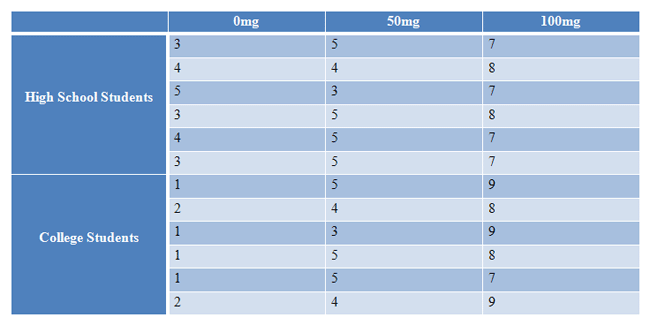
Figure 1.

Let's try a full example:

Steps for Factorial ANOVA, Two Independent Factors
1. Define Null and Alternative Hypotheses 2. State Alpha 3. Calculate Degrees of Freedom 4. State Decision Rule 5. Calculate Test Statistic 6. State Results 7. State Conclusion

1. Define Null and Alternative Hypotheses

Here, we have three. One for each main effect, and one for the interaction.

Figure 2.

2. State Alpha

alpha = 0.05

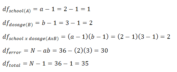
3. Calculate Degrees of Freedom

Degrees of freedom are calculated as follows. "a" is the number of a groups you have, "b" is the number of b groups you have, and "N" is your total number of scores.

Figure 3.

4. State Decision Rule

We have three hypotheses, so we have three decision rules. Critical values are found using the effect and error degrees of freedom for our three effects:

Figure 4.

We now head to the F-table and look up our critical values using alpha = 0.05. In the table, we find the critical values shown below:

Figure 5.

These critical values bring us to our three decision rules:

[School] If F is greater than 4.17, reject the null hypothesis.

[Dosage] If F is greater than 3.32, reject the null hypothesis.

[Interaction] If F is greater than 3.32, reject the null hypothesis.

5. Calculate Test Statistic

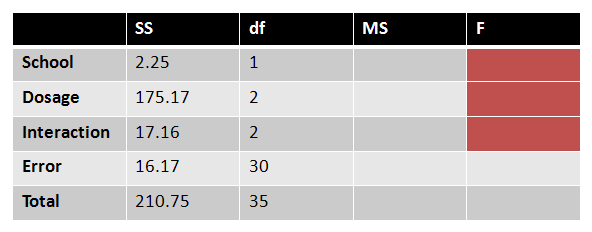
First, we'll put the degrees of freedom that we've already calculated into our source table:

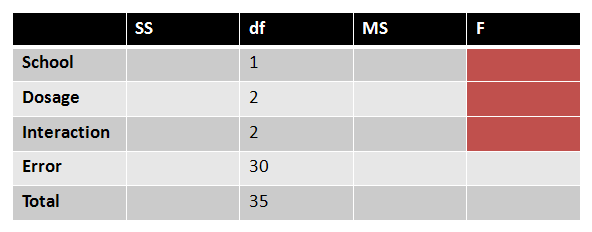
Figure 6.

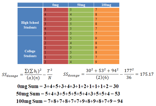
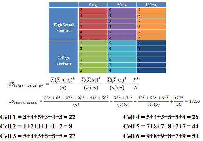
Next, we need to find the five SS values we are missing:

Figure 7.

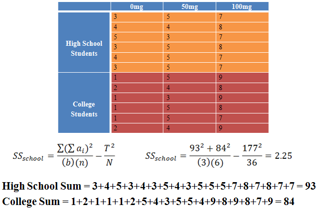
Figure 8.

Figure 9.

Figure 10.

Figure 11.

These SS values are then placed into our source table. We find the last missing SS value by subtracting everything we've found so far from the total.

Figure 12.

Each MS value is found by dividing each SS by their respective degrees of freedom:

Figure 13.

Finally, our three F values are found:

Figure 14.

6. State Results

[School] If F is greater than 4.17, reject the null hypothesis.

Our F = 4.166. Retain the null hypothesis.

[Dosage] If F is greater than 3.32, reject the null hypothesis.

Our F = 162.20. Reject the null hypothesis.

[Interaction] If F is greater than 3.32, reject the null hypothesis.

Our F = 15.89. Reject the null hypothesis.

7. State Conclusion

High school students and college students did not have significantly different anxiety levels, F(1, 30) = 4.166, p > 0.05. There was a significant difference between the three different levels of dosage, F(2, 30) = 162.20, p < 0.05. An interaction effect was also present, F(2, 30) = 15.59, p < 0.05.

---